The obstacle
Euclidean distortion
A matrix may have all eigenvalues on the unit circle and still stretch some vectors in the usual Euclidean norm. Eigenvalue magnitudes do not by themselves determine whether lengths and angles are preserved.
What if the operator is fixed, but the geometry is ours to design? An exact existence and classification theory for Hilbert-space geometries in which a prescribed linear operator becomes norm preserving.
Choose a geometry first, then ask whether an operator respects it.
Fix the operator first, then construct a compatible RKHS geometry.
Most representation-learning methods modify features or fit a new transformation. This work reverses the question: given an operator, can we design the inner product—and therefore an RKHS—in which that operator acts as an exact isometry?
A matrix may have all eigenvalues on the unit circle and still stretch some vectors in the usual Euclidean norm. Eigenvalue magnitudes do not by themselves determine whether lengths and angles are preserved.
Instead of altering the dynamics, choose a Hermitian matrix \(G\succ0\) that defines the inner product. Exact invariance is expressed by \(M^*GM=G\).
Each admissible metric induces a reproducing kernel on the chosen feature space. The question is not merely whether a solution exists, but how to characterize all compatible geometries.
A vector norm is not intrinsic to its coordinate entries: it depends on the inner product. In standard coordinates we use \(\|c\|_2^2=c^*c\); in a feature-space geometry we can instead use \(\|c\|_G^2=c^*Gc\). Thus, the statement that a transformation “preserves length” must always specify which length.
Requiring this to equal \(\|c\|_G^2\) for every coefficient vector \(c\) yields the fundamental equation \(M^*GM=G\). This is the bridge from an intuitive geometric question to a precise matrix problem.
Start with an ordinary rotation \(R_\theta\), which preserves Euclidean length. Let \(S\) be invertible, and describe the same motion in distorted coordinates by \(M=SR_\theta S^{-1}\). In general \(M^*M\ne I\): Euclidean circles can appear stretched even though the underlying dynamics are rotational.
With this adapted metric, \(M^*GM=G\) exactly. The geometry compensates for the coordinate distortion without changing the operator. Section 05 lets you vary the rotation and shear and observe this construction.
In a finite-dimensional feature space, a function is represented by coefficients in a basis of features. A positive-definite Gram matrix determines their inner products, while its inverse appears in the corresponding reproducing kernel. Designing \(G\) therefore changes not only a matrix norm but the Hilbert-space geometry of the represented functions.
This makes the inverse problem relevant to representation learning: we seek feature-space geometries in which a prescribed linear action has a guaranteed structural property, rather than relying on an unconstrained learned representation.
Changing the inner product cannot erase genuine exponential growth, decay, or a nontrivial Jordan block. In finite dimensions, an invertible matrix admits a positive-definite solution of \(M^*GM=G\) if and only if it is diagonalizable over \(\mathbb C\) and all of its eigenvalues lie on the unit circle. This criterion separates geometries that can be designed from operators for which exact isometry is impossible.
The equivalence is for the finite-dimensional setting studied here; it is not a blanket statement about arbitrary infinite-dimensional operators.
When the criterion holds, an adapted RKHS can encode exact norm preservation under the specified operator. This gives a principled geometric ingredient for stable operator representations, invariant feature dynamics, and controlled comparisons of learned coordinates.
These are motivations and possible uses of the construction, not claims that the paper establishes improved performance for every downstream learning task.
Rather than checking whether a fixed kernel happens to make \(M\) isometric, we ask which kernels do. The admissible set of metrics can contain many choices; their classification reveals freedom to tailor a representation while preserving the same exact operator identity.
A prescribed linear operator \(M\).
Can \(M\) preserve a positive-definite inner product?
Find and classify \(G\succ0\) satisfying \(M^*GM=G\).
Construct the corresponding RKHS kernels \(k_G\).
The central mathematical step is to translate a question about preserving the norm of functions into a matrix equation for the inner product. This section follows Proposition 2.1, Theorem 2.2, and Remark 2.3 of the accepted manuscript, with short derivations explaining why each condition matters.
Choose linearly independent complex-valued functions \(\psi_1,\ldots,\psi_m\) on a nonempty set \(X\). Their span is a finite-dimensional function space. The prescribed linear operator \(T\) acts on coefficient vectors through a matrix \(M\).
The coefficients \(c\) describe a function, but they do not determine how its length is measured. That additional choice is encoded by a Hermitian positive-definite matrix \(G\).
Positive definiteness ensures that every nonzero function has positive squared norm. Changing \(G\) changes the geometry without changing the basis functions or the action of \(T\).
Proposition 2.1. Every \(G\succ0\) yields a reproducing-kernel Hilbert space on the same finite-dimensional function space. The inverse matrix appears because kernel sections must represent point evaluation under the chosen inner product.
For a fixed \(y\in X\), the kernel section \(k_G(\cdot,y)\) has coefficient vector \(G^{-1}\Psi(y)\). Using the inner-product convention in the manuscript,
This is the reproducing property. It makes the connection between a positive-definite matrix and a genuine function-space kernel exact—not merely an analogy with metric learning.
Since \(Tf_c=f_{Mc}\), asking the operator to preserve the RKHS norm for every function is equivalent to asking that a quadratic form remain unchanged for every coefficient vector:
Theorem 2.2. This equation is necessary and sufficient for \(T\) to act isometrically on the constructed RKHS. It is a linear matrix constraint in the unknown entries of \(G\), together with the essential requirement \(G\succ0\).
Theorem 2.2 further shows that a positive-definite solution exists if and only if \(M\) is similar to a unitary matrix. In finite dimensions, this is equivalent to two simultaneous requirements:
Unit-modulus eigenvalues are necessary, but they are not sufficient on their own.
Every eigenvalue of \(J\) equals one, yet its powers grow. If \(J^*GJ=G\) held for a positive-definite \(G\), all powers would preserve the \(G\)-norm—contradicting this growth. A nontrivial Jordan block therefore obstructs exact adaptation.
Suppose \(M=SDS^{-1}\), where \(S\) is invertible and \(D\) is diagonal with unit-modulus entries. Then \(D^*D=I\). Choose
This \(G\) is positive definite, and direct substitution gives
Conversely, if \(M^*GM=G\), then \(U=G^{1/2}MG^{-1/2}\) satisfies \(U^*U=I\). Hence \(M\) is similar to a unitary matrix. These two directions explain the exact existence criterion.
Once the metric equation holds, the operator preserves pairwise inner products and the corresponding distances and angles in the adapted Hilbert geometry.
The construction applies to a fixed finite-dimensional invariant function space and a prescribed linear action on it. It does not imply that arbitrary dissipative, unstable, defective, or infinite-dimensional operators admit an exact positive-definite invariant RKHS metric.
Existence is only the first question. Once a prescribed operator admits an invariant inner product, which positive-definite metrics preserve it, how many free parameters remain, and what kernels do they produce? Theorem 2.4 and Corollaries 2.5–2.6 answer these questions in the finite-dimensional setting.
Section 02 constructed one solution when the operator is diagonalizable with unimodular eigenvalues. But that construction is not unique: changing the inner product within invariant eigenspaces can preserve exactly the same operator. The classification determines all such choices.
Write \(M=SDS^{-1}\), where \(D=\operatorname{diag}(\mu_1 I_{m_1},\ldots,\mu_r I_{m_r})\), the \(\mu_j\) are distinct, and \(|\mu_j|=1\). Define \(H=S^*GS\). Then the invariance equation becomes
Because \(S\) is invertible, \(G\succ0\) if and only if \(H\succ0\). Thus no admissible metric is lost by working in eigen-coordinates.
Partition \(H\) into blocks \(H_{ij}\) matching the eigenspaces. The invariance identity reads
If \(i\neq j\), the eigenvalues are distinct and unimodular, so \(\overline{\mu_i}\mu_j\neq1\). Hence \(H_{ij}=0\). Within a repeated-eigenvalue block, however, the equation imposes no additional restriction beyond Hermitian positive definiteness.
Here \(S^{-*}=(S^{-1})^*\). Each positive-definite block \(H_j\) may be chosen freely, and every solution of \(M^*GM=G\) arises in this way. The metric from Section 02 is recovered by setting every \(H_j=I_{m_j}\).
Consequently, classification of invariant inner products gives a corresponding family of reproducing kernels for the same finite-dimensional function space. The feature functions \(\Psi\) are held fixed; what changes is their Hilbert-space geometry.
If all \(n\) eigenvalues are distinct, each block is \(1\times1\):
The family has \(n\) real parameters. Geometrically, the eigen-directions can be weighted independently, but distinct eigenspaces cannot acquire cross terms in eigen-coordinates.
An eigenspace of complex dimension \(m_j\) allows any \(m_j\times m_j\) Hermitian positive-definite matrix. This includes off-diagonal correlations between eigenvectors sharing the same eigenvalue.
This counts real parameters in the cone of Hermitian invariant metrics on a complex function space. It is not the count for a separately constrained real-symmetric metric family.
Consider the diagonal unitary operator below, with two equal eigenvalues and a third distinct eigenvalue:
Its invariant metrics in eigen-coordinates are exactly
The free variables are \(a,b,c\in\mathbb R\) and \(z\in\mathbb C\): five real parameters, agreeing with \(2^2+1^2=5\). If the three eigenvalues were distinct, the off-diagonal \(z\) would be forced to zero and the dimension would drop to three.
For \(M=\mu I_n\) with \(|\mu|=1\), every Hermitian positive-definite \(G\) is invariant, yielding \(n^2\) real parameters. At the opposite extreme, a simple spectrum allows only \(n\) independent positive weights in the eigenbasis.
The dimension counts a family of metrics, not the number of independent eigenvalues or a learned model's parameter count.
If \(G\in\mathcal G(M)\), then \(cG\in\mathcal G(M)\) for every \(c>0\). Thus even the overall metric scale is not determined by isometry alone. Additional design criteria or a normalization (for example, fixing \(\operatorname{tr}G\)) can select among admissible geometries.
A normalization reduces the available freedom; it is not part of the invariant-metric equation itself.
The classification gives a feasible family of RKHS geometries in which the prescribed operator is exactly norm-preserving. Within that family, one may subsequently investigate conditioning, interpretability, or compatibility with data without sacrificing the identity \(M^*GM=G\).
This is a mathematical design opportunity, not a claim that the paper proves a particular data-driven criterion will choose the best kernel or improve downstream accuracy.
The numerical verification isolates the central claim of the paper: an operator can be spectrally stable yet fail to preserve Euclidean geometry. Changing the inner product—not the underlying operator—restores an isometric representation.
A synthetic linear operator similar to a unitary matrix, but non-unitary in the native Euclidean metric.
Normalized pairwise kernel-invariance error in Euclidean geometry.
Near machine precision after using the operator-adapted metric.
The manuscript constructs a 20-dimensional operator \(M\) that is similar to a unitary matrix. Its eigenvalues lie on the unit circle, but its Euclidean singular values need not equal one. A positive-definite matrix \(G\) is constructed so that \(M^*GM=G\). Equivalently, the matrix below is unitary:
Similarity preserves the eigenvalues, not the singular values. The latter depend on the chosen inner product, which is exactly what this experiment tests.
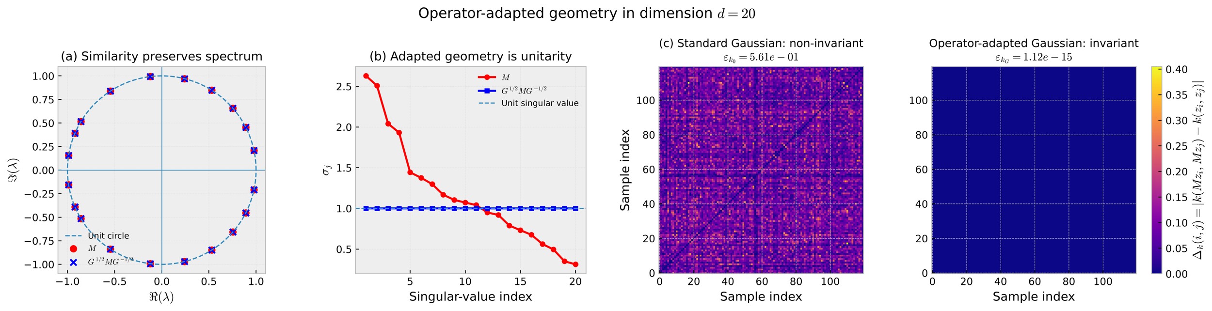
Figure 1 from the accepted manuscript. Panel (a) compares the unchanged spectra; panel (b) contrasts singular values in Euclidean and adapted coordinates; panels (c) and (d) compare pairwise kernel-invariance discrepancies using a common color scale. The figure is reproduced from the supplied accepted paper.
When \(M\) is non-unitary in Euclidean coordinates, it can alter distances \(\|Mx-My\|_2\), and therefore change Gaussian similarities. Unit-modulus eigenvalues alone do not prevent this.
Because \(M^*GM=G\), the squared adapted distance is unchanged under \(M\), giving \(k_G(Mx,My)=k_G(x,y)\) exactly in mathematics.
With \(N=120\) sampled vectors \(z_1,\ldots,z_N\in\mathbb R^{20}\) and bandwidth \(\gamma=3\), the paper measures every pairwise change in similarity:
Thus \(\varepsilon_k=0\) means all sampled pairwise kernel values are preserved. The reported adapted value \(1.12\times10^{-15}\) is a finite-precision numerical confirmation of the exact invariance identity.
The spectral plot cannot distinguish the two geometric descriptions, but the singular-value comparison and kernel discrepancy can. This supports the paper's central inverse-design perspective: preserve the operator and choose a compatible RKHS geometry.
This is a controlled linear-algebra experiment, not a trained neural-network benchmark or an evaluation of downstream forecasting accuracy. The numerical result validates the construction for the chosen operator and sampled representations; the general existence and classification statements come from the theorems.
This self-contained 2D illustration shows exactly how an adapted positive-definite metric converts a non-orthogonal similarity transform of a rotation into an isometry. It is not a reproduction of the paper's 20D numerical experiment.
Construct \(S=\begin{bmatrix}1&s\\0&1\end{bmatrix}\), \(M=S R_\theta S^{-1}\), and \(G=S^{-T}S^{-1}\). This guarantees \(M^TGM=G\) for every slider setting.
Dashed outlines show the image of each unit curve under \(M\). The Euclidean circle generally changes shape, while the \(G\)-unit ellipse maps onto itself.
Norm preservation is exact because the metric is constructed from the similarity transform. The Euclidean matrix need not be orthogonal.
Consequently, every Gaussian kernel using this invariant quadratic form preserves pairwise similarity under the transformation.
The mathematical statements and reported numerical values on this site are taken from the accepted manuscript. The interactive illustration is a separate, analytically exact teaching example.
Himanshu Singh · NeurIPS 2026 GlobalSouthAI
Open paper PDF ↗Explore the code, experiment settings, and related research artifacts in the linked repository. The site's browser demo does not require a Python environment.
Visit GitHub ↗The existence and classification results concern finite-dimensional function spaces. The paper identifies extension to infinite-dimensional RKHSs, including bounded positive invertible metric operators, as a separate research direction. The 2D web demonstration is not an additional empirical result.
Singh, H. (2026). Operator-Adapted Reproducing Kernel Geometries for Structure-Preserving Representation Learning. NeurIPS 2026 GlobalSouthAI. Verify the final proceedings metadata and URL before using a formal BibTeX entry.