Symmetry and Geometry in Neural Representations
Kernelized Koopman Representation Geometry Governs Transient Amplification in Neural Dynamical Systems
The same neural dynamics can yield dramatically different finite-time behavior when represented in different reproducing kernel Hilbert spaces.
Illustrative curves only. The laboratory below displays numerical results from the research repository.
Two models can reproduce the same neural trajectories yet respond very differently in representation space.
Data-driven Koopman models are often evaluated through prediction error, reconstructed spectra, and eigenfunctions. But these diagnostics do not, by themselves, characterize how a learned operator behaves over finite time.
Stable-looking spectra are not enough
Non-normal operators may exhibit large transient growth even when their eigenvalues suggest asymptotic stability. Such amplification can affect correlations and perturbation-response calculations.
A kernel chooses a geometry
Kernel Extended Dynamic Mode Decomposition (KEDMD) represents observables in a reproducing kernel Hilbert space. Different kernels induce different Gram matrices, norms, and finite-dimensional surrogate operators.
Is a Koopman surrogate representation-neutral?
Given the same neural dynamics and snapshot pairs, how does kernel choice alter finite-time operator growth, correlation amplification, and resolvent sensitivity?
Beyond eigenvalues
We examine regularized KEDMD surrogates using Gram-induced operator norms, correlation-based transient amplification, pseudospectra, and grid-based Kreiss constant estimates. The study compares four kernels across linear excitatory–inhibitory, Wilson–Cowan, and FitzHugh–Nagumo dynamics.
Representation quality is dynamical
Two kernel surrogates should not be treated as interchangeable merely because they use the same trajectories or have similar spectra. Before using a surrogate for prediction or perturbation-response analysis, we should inspect its finite-time amplification and resolvent behavior.
Scope: these findings concern finite-dimensional, regularized kernelized Koopman representations; they do not imply that the physical neural dynamics themselves change when a kernel is changed. This motivation follows the accepted paper's Introduction and problem statement.
Eigenvalues alone do not tell the whole story.
Kernel choice changes the geometry in which a data-driven Koopman surrogate is measured. Even with nearly unit spectral radii, the resulting finite-time operator growth can differ substantially.
Identical physical dynamics
Compare kernelized representations learned from the same underlying neural dynamical system.
Distinct induced geometries
Each positive-definite kernel determines a different feature geometry and associated Gram matrix.
Non-normal amplification
Representation-dependent transient growth becomes visible through induced norms and pseudospectral diagnostics.
Representation-space maximum
Same physical system and snapshot pairs
Linear E–I · Wilson–Cowan · FitzHugh–Nagumo
Four kernels. Four ways of measuring similarity.
The kernel is not merely a computational ingredient: it specifies the inner-product geometry of the sampled representation. The four families below are exactly those used in the accompanying kernel-section visualization code.
How to read the original scientific figure. Color encodes similarity to the anchor \(z_0=(0.88,0.14)\); white curves are the \(0.2,0.4,0.6,0.8\) similarity contours; white arrows point along \(+\nabla_x k(x,z_0)\), toward increasing similarity. The code uses a common maximum gradient magnitude for cross-kernel arrow scaling, followed by square-root compression and a minimum display length. These arrows are kernel gradients, not trajectories of the neural dynamical system.
Laplace · \(L^1\) distance
Diamond-shaped similarity contours arise from the sum of absolute coordinate differences. The section is not differentiable along coordinate lines passing through the anchor.
Interpretation: coordinatewise sensitivity and sharp local similarity. This is the specific \(L^1\)-Laplace variant used by the supplied plotting code.
Matérn-3/2
Circular contours and a smooth first derivative reflect radial similarity with limited smoothness relative to the Gaussian.
Interpretation: a balance of locality and regularity; not a guarantee of better numerical conditioning.
Rational Quadratic
Algebraic tails retain similarity farther from the anchor than exponentially decaying sections. The shape parameter \(\alpha\) changes the relative contribution of spatial scales.
Interpretation: multiscale radial coupling. The original figure uses \(\alpha=1\).
Gaussian RBF
Its circular contours reflect Euclidean radial similarity and rapid decay away from the anchor. The corresponding RKHS consists of highly regular functions.
Interpretation: smoothness is a function-space property, not a promise of low transient amplification.
Change the bandwidth and anchor. Watch the geometry respond.
The four panels are generated interactively from the mathematical kernel definitions used in the accompanying Python visualization. Adjusting the parameters changes the kernel similarity fields and their contours; it does not retrain the Koopman model or recompute transient amplification.
Shared color mapping: dark = low similarity, mint/gold = high similarity. White curves show equal-similarity levels (0.2, 0.4, 0.6, 0.8); the white dot is the anchor. These live panels omit gradient arrows to keep the geometry readable while parameters change. The original research figure above retains the analytic gradient normals.
Why this matters for Koopman representations
Given sampled states \(x_1,\ldots,x_m\), each kernel determines a Gram matrix \(G_k=[k(x_i,x_j)]\). With regularization, the corresponding normalized fitted operator is
The same physical dynamics can have different fitted kernel representations and different measured finite-time growth. Contour shape alone does not establish an amplification ranking; that evidence comes from the KEDMD experiments and Kreiss analysis.
Explore representation-dependent transient amplification.
Switch between neural dynamical systems and kernel representations. The peak gains, peak times and spectral radii below are loaded from the original CSV results in the repository.
Linear excitatory–inhibitory dynamics
Peak \(g_{\max}=\max_t\|A_\lambda^t\|_{G_\lambda}\). Bars use a shared 0–17× scale across all systems.
1.0000
0.50
1.65 × 10³
1.2257
Values refer to regularized finite-dimensional KEDMD surrogates, not intrinsic amplification of the infinite-dimensional Koopman operator.
Measured transient-growth curves
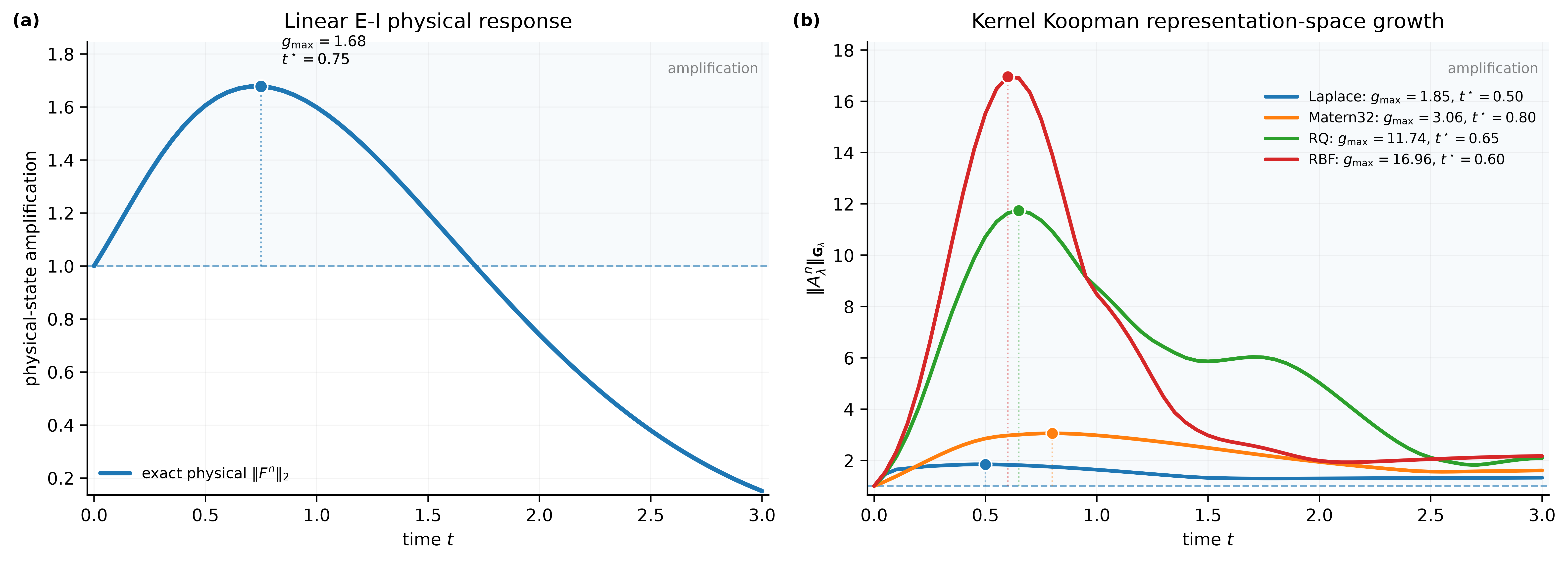
Published full curves; switch system above to change the figure.
Corresponding pseudospectra
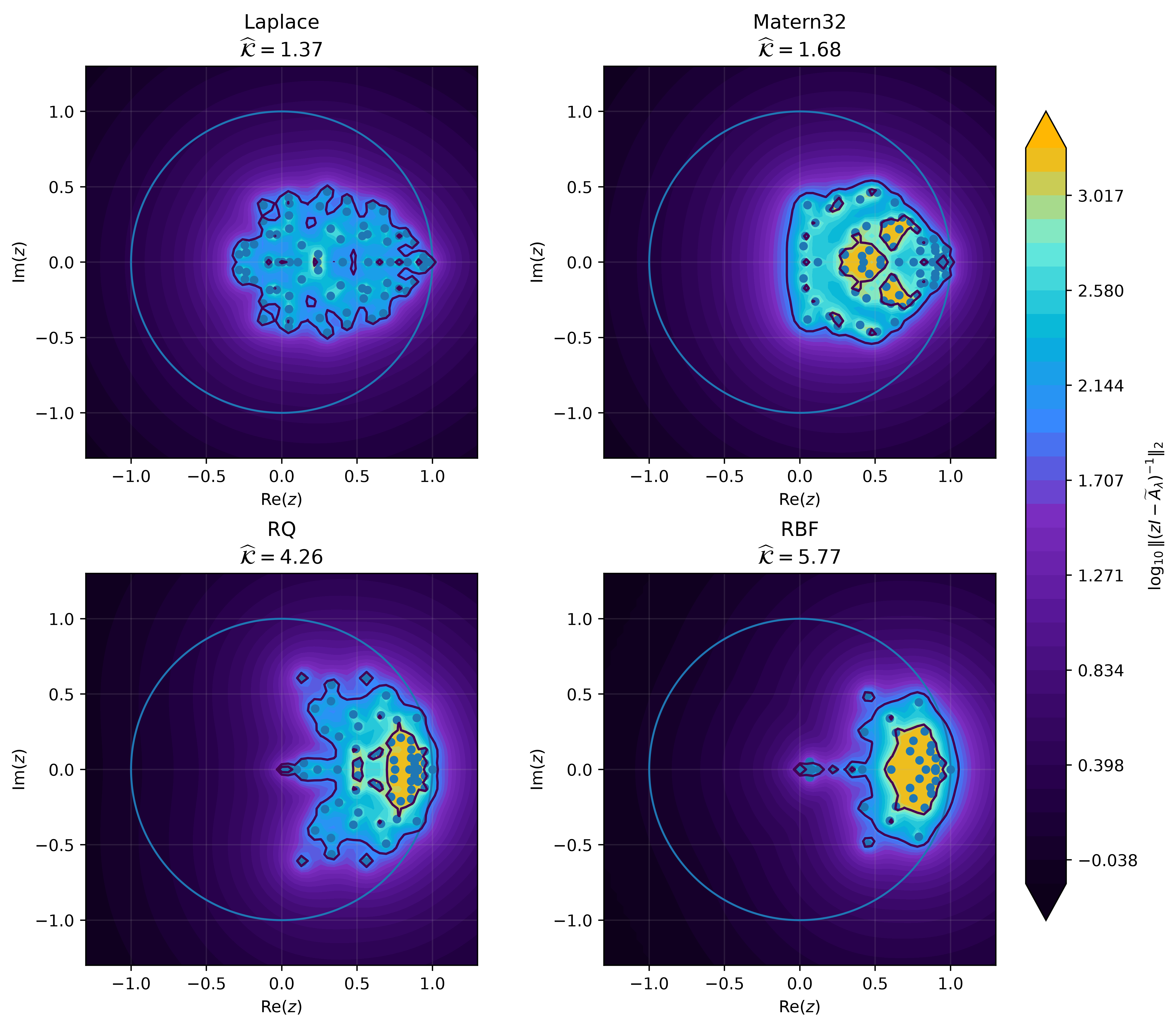
Published pseudospectral contours for the selected system.
Why does kernel geometry govern transient amplification?
The theory answers a sequence of questions: how the same physical map transports kernel sections, how the resulting geometry enters a finite-dimensional Koopman approximation, and why that representation can exhibit large short-time growth even when its eigenvalues look benign.
Prediction and eigenvalues do not tell the whole story.
Consider the same neural system, the same observed snapshot pairs, and several different kernels. A kernel changes the RKHS in which the data are represented, the associated Gram matrix, and the fitted KEDMD surrogate. Consequently, two surrogates may have similar spectral locations but very different norms of their powers. The central mathematical task is to trace this discrepancy from kernel geometry to operator growth and finally to observable correlations.
The analysis concerns finite-dimensional learned representations. A large surrogate norm does not, by itself, imply a comparably large physical-state perturbation or an instability of the original neural dynamics.
From state evolution to kernel coordinates
The physical system evolves as \(x_{t+1}=F(x_t)\). Its Koopman operator acts on observables, \((Uf)(x)=f(F(x))\). The RKHS reproducing identity \(\langle f,k_x\rangle_{\mathcal H_k}=f(x)\) leads, under the paper's domain assumptions, to the kernel-section transport relation
Why this matters: it converts the evolution of an observable into a statement about how kernel sections move. The before-and-after Gram matrices then measure this deformation without requiring a global coordinate system for the full RKHS.
Compare geometry before and after the same dynamics.
For the snapshot sets \(X=\{x_i\}\) and \(Y=\{F(x_i)\}\), the matrices \(G_X\) and \(G_Y\) encode pairwise kernel-section inner products. The map \(T_{F,X}\) carries each section \(k_{x_i}\) to \(k_{F(x_i)}\). Its squared norm is the largest possible ratio of transported to initial RKHS energy:
The maximization of this quotient motivates Proposition 5. The result is a generalized eigenvalue problem, not a claim that the physical dynamics changed when the kernel changed.
Euclidean coefficient length is not RKHS function length.
The coefficient vector \(v\) represents a kernel expansion, whose geometry is measured by \(\|v\|_{G_\lambda}^2=v^*G_\lambda v\), rather than by \(v^*v\). Regularization makes \(G_\lambda=G_X+\lambda I\) positive definite. The coordinate change \(u=G_\lambda^{1/2}v\) converts the induced norm into an ordinary matrix 2-norm:
Why this matters: the normalized operator is the object whose transient growth, pseudospectra, and Kreiss constant can be compared consistently in the induced geometry. This is the central change of coordinates in Theorem 10.
Connect operator growth to an observable quantity.
The paper begins with time correlations of observables, then introduces their finite-dimensional KEDMD counterpart \(C_f^{(\lambda)}(t)=v^*G_\lambda A_\lambda^t v\). Cauchy–Schwarz bounds the correlation magnitude by the initial coefficient energy multiplied by the induced operator growth.
Interpretation: the operator norm bounds the worst-case response, but a particular observable need not attain it. Corollary 11 sharpens the connection by identifying the supremum of normalized self-correlations with the numerical radius.
Spectral stability is not a finite-time growth guarantee.
For a normal normalized matrix, the norm of its powers is determined by its spectral radius. A non-normal matrix can have eigenvalues inside the unit disk while its powers first grow and only later decay. This motivates two complementary diagnostics: direct finite-time power norms and resolvent-based pseudospectral analysis.
Theorem 10 connects these quantities under stated hypotheses. The Kreiss laboratory then tests the distinction using numerical estimates from the three neural-system experiments.
The precise mathematical statements.
The cards below collect the results in the order used in the paper. The explanations above provide the motivation; these formulas state what is actually proved or bounded.
Geometry deformation under the same physical map
On the sampled span \(V_X=\mathrm{span}\{k_{x_i}\}\), the section-transport map sends \(\sum_i c_i k_{x_i}\) to \(\sum_i c_i k_{F(x_i)}\). For invertible \(G_X\),
Proof idea. The squared ratio of image and source RKHS norms is \(c^*G_Yc/(c^*G_Xc)\); maximize the generalized Rayleigh quotient. If \(G_X\) is singular, well-definedness and pseudoinverse treatment require additional conditions.
The geometry-sensitive transport factor
This factor measures regularized transport deformation. It enters the normalized KEDMD growth bound below.
Observable-level amplification
For \(C_f^{(\lambda)}(t)=v^*G_\lambda A_\lambda^t v\), the induced norm gives
This follows from Cauchy–Schwarz in the \(G_\lambda\) inner product and the definition of the induced operator norm.
Why the kernel-induced norm matters
When \(\widetilde A_\lambda\) is normal, \(\|\widetilde A_\lambda^t\|_2=\rho(\widetilde A_\lambda)^t\). For non-normal surrogates, eigenvalues alone do not control finite-time growth.
The Kreiss and pseudospectral implications of Theorem 10 are developed in the dedicated laboratory below. The finite-dimensional Kreiss upper bound requires the spectrum to lie in the closed unit disk.
Normalized correlation response
The equality follows by the change of variables \(u=G_\lambda^{1/2}v\); the inequality uses the numerical radius bound.
The resolvent reveals what the spectrum conceals.
Unlike a spectral-radius diagnostic, the Kreiss quantity responds to non-normal resolvent amplification. Here we use the paper's grid-based estimates, and retain the exact distinction between the sampled numerical maximum and the continuous Kreiss constant.
Resolvent and power growth
For an \(n\times n\) matrix with spectrum in the closed unit disk. Some fitted surrogates in the paper have spectral radii slightly above one, so the right-hand finite upper bound must not be applied to those matrices without modification.
Outward pseudospectral inflation
Here \(r_\varepsilon\) is the radial extent of the \(\varepsilon\)-pseudospectrum. This lower bound is informative when the pseudospectrum extends beyond the unit circle.
Resolvent sensitivity vs. transient amplification
| Kernel | Peak growth | K̂ (61²) | K̂ (121²) | ρ(Ã) | r₀.₀₁ |
|---|
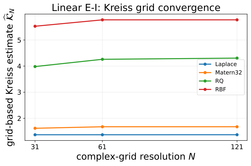
All values are sourced from the repository's transient, pseudospectral and grid-convergence CSV files. The 61×61 estimates correspond to the main paper's Table 2; the 121×121 values provide a refinement check (Appendix D).
Grid-resolution convergence
Pseudospectral contours
How the estimates were computed
Construct \(\widetilde A_\lambda\), sample \(z\) on a Cartesian grid over \([-1.3,1.3]^2\), retain \(|z|>1\), evaluate \(\sigma_{\min}(zI-\widetilde A_\lambda)\), then maximize \((|z|-1)/\sigma_{\min}\).
The study checks 31×31, 61×61 and 121×121 grids. The paper reports that 61→121 refinement changes estimates by at most approximately 1.1%, with the kernel ordering preserved.
Kreiss is not the transient peak
The discrete Kreiss estimate is a resolvent diagnostic, not a direct prediction of the peak power norm. The kernel ordering agrees across these experiments, but numerical values differ and the true supremum is not generally attained on the finite grid.
A finite-horizon peak is also not necessarily the infinite-horizon supremum appearing in the Kreiss matrix theorem.
How can a spectrally stable system amplify a perturbation?
This is a controlled two-dimensional matrix example, not a measurement from the neural-system experiments. It isolates non-normal coupling, the mechanism behind transient growth, while keeping every eigenvalue fixed.
Does a stable spectrum guarantee that every perturbation immediately decays?
No. Eigenvalues determine asymptotic stability, but the singular values of matrix powers determine the largest finite-time amplification of an initial perturbation. Those are different mathematical questions.
Both eigenvalues are always 0.8. The parameter \(\alpha\) changes only the off-diagonal coupling. When \(\alpha=0\), the operator is normal and every state contracts by \(0.8\) per step. When \(\alpha\neq0\), the matrix is non-normal, and its coordinate coupling can temporarily transfer energy into an amplified direction.
Predicts eventual decay as \(t\to\infty\), not monotone decay at each step.
Largest possible \(\|B_\alpha u_0\|_2/\|u_0\|_2\) over unit vectors \(u_0\).
A unit right singular vector of \(B_\alpha^{t_*}\). The vector orientation matters, not only the eigenvalues.
The worst-case perturbation at each time
The plotted curve is not one arbitrary trajectory. At each time \(t\), it measures the maximum amplification over all unit initial perturbations. The maximizing direction can depend on time.
A polynomial factor competes with exponential decay
The off-diagonal term initially grows in proportion to \(t\), while the factor \(0.8^{t-1}\) eventually decays. Their competition creates a finite-time peak even though every eigenvalue lies strictly inside the unit circle.
Eigenvalues alone are incomplete
Move the slider from \(\alpha=0\) to a positive value. The spectral radius remains \(0.8\), but the largest singular value of a matrix power can become greater than one. A system can therefore be asymptotically stable yet strongly amplify some perturbations before they decay.
It is a mechanism, not a kernel comparison
The matrix \(B_\alpha\) is a synthetic example in Euclidean geometry. It does not compute a kernel Gram matrix, fit KEDMD, or reproduce any numerical amplification values from the paper. Its purpose is to make the spectral-versus-transient distinction transparent.
From a 2×2 example to kernelized Koopman representations
In the paper, the finite-dimensional fitted operator is assessed in a kernel-induced geometry, rather than by treating arbitrary coefficient coordinates as intrinsically Euclidean. The relevant normalized matrix takes the form
The illustration explains why we measure powers of the normalized operator and examine non-normality: a stable spectrum by itself does not determine the transient response. The experiments, rather than this toy model, establish how that response varies across kernels and neural systems.
Takeaway: Spectral stability concerns the long run. Transient amplification concerns the largest possible short-run response. Kernel geometry affects the latter through the fitted representation and its norm.
Which kernel is preferable when several criteria matter?
Kernel choice changes both the learned dynamics and the numerical geometry of the representation. Rather than declare one universally best kernel, the experiments compare configurations by finite-time gain, early observable response, and Gram-matrix conditioning. The three original figures below show the empirical trade-offs for linear excitatory–inhibitory, Wilson–Cowan, and FitzHugh–Nagumo dynamics.
A single metric can conceal a trade-off.
Suppose configuration A has smaller transient amplification but larger early observable response than configuration B. Neither is uniformly preferable on those two objectives. Pareto analysis distinguishes such trade-offs from configurations that are worse in both measurements.
A configuration is empirically Pareto nondominated when no other sampled kernel–regularization pair dominates it. “Empirical” matters: the frontier is defined only over the finite configurations actually tested, not over every possible kernel and parameter value.
Control transient and observable response
Horizontal: peak finite-time KEDMD amplification in the regularized Gram-induced norm. Vertical: peak magnitude of the early observable-correlation response, for the system-specific observable.
Smaller values lie toward the lower-left. The early-response objective is a quantity to be minimized in these scripts; it should not be confused with a forecast skill score for which larger would be better.
Balance conditioning against amplification
The inset asks whether a low-gain configuration is also numerically well conditioned. Here \(\kappa(G_\lambda)\) is the condition number of the regularized kernel Gram matrix.
The dynamical and numerical frontiers are computed separately. A point can belong to one frontier without belonging to the other.
Linear excitatory–inhibitory · Pareto dominance
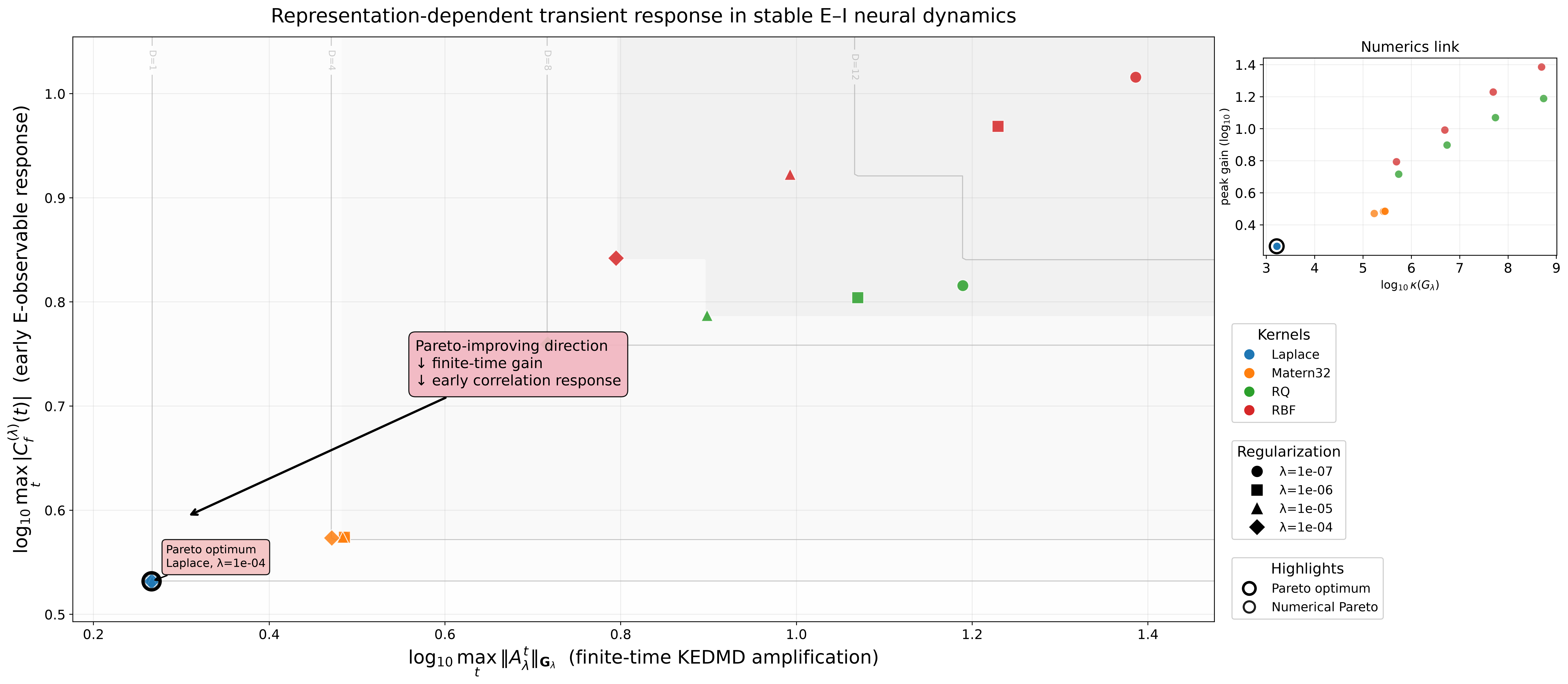
Linear E–I: the main plane compares peak KEDMD gain against the early excitatory-observable response. The inset compares Gram conditioning against gain. Original figure from the research repository.
Each marker is a tested configuration
Color identifies the kernel family: Laplace, Matérn-3/2, Rational Quadratic, or Gaussian RBF. Marker shape identifies the regularization level \(\lambda\), with levels obtained from each system's own sweep. Outlined points indicate membership in a Pareto set.
The line connecting dynamical Pareto points is a visual guide through sampled nondominated configurations, not a continuously optimized theoretical frontier.
Dominance depth is a count, not a density
At a location \((x,y)\), \(D\) counts sampled configurations that are no worse in either objective. A larger depth indicates that more tested alternatives lie down-and-left of that location.
The figure's shaded regions and labeled \(D\)-contours visualize this dominance count. They do not measure probability, uncertainty, or sample density.
Linear excitatory–inhibitory · What is being compared?
The E–I sweep evaluates kernel and regularization choices on peak KEDMD amplification and the early response of an excitatory observable. The numerical inset tests whether reduced amplification comes with a better-conditioned regularized Gram matrix.
Compare points within this system's own sweep. Do not interpret the log axes as direct comparisons of physical units across different neural models.
Find the lower-left boundary
Configurations on the empirical dynamical Pareto frontier cannot improve one plotted dynamical objective without worsening the other, among the tested choices. Configurations above and to the right of another point are dominated and can be rejected for this pair of objectives.
Compare the inset, not just the main panel
A configuration with attractive dynamical response may still have an ill-conditioned Gram matrix. The numerical frontier makes this visible instead of folding conditioning into an arbitrary weighted score.
Follow regularization, not just kernel color
Each point represents a kernel–regularization pair. Changing \(\lambda\) can alter conditioning, fitted dynamics, and transient gain; a single kernel family may therefore occupy several distinct regions of the objective plane.
Check whether the conclusion transfers
Use the system selector to compare the three experiments. A configuration that is nondominated for one neural system need not be nondominated for another. Pareto membership is relative to the chosen system, objectives, and sampled sweep.
How the plotted frontiers were constructed
The supplied scripts load each system's mechanistic-sweep CSV, compute base-10 logarithms of the positive diagnostics, identify nondominated points by pairwise minimization, and calculate the dominance-depth field over a two-dimensional grid. The dynamical frontier uses peak_G and corr_peak; the numerical frontier uses cond_G or cond_Glambda and peak_G.
Because logarithms are monotone on positive values, applying \(\log_{10}\) does not change the Pareto ordering of valid positive observations. The scripts use a small positive floor when forming logs; the underlying data should be checked for nonpositive or missing diagnostics before interpreting the results.
Selection principle: Use the Pareto set to eliminate jointly inferior sampled choices, then choose among nondominated configurations according to the scientific importance of observable response, transient growth, and numerical conditioning. This is a diagnostic selection framework, not a theorem that one kernel family is universally optimal.
Related sections: finite-time growth laboratory · Kreiss and pseudospectral analysis · source repository ↗
Learn the mathematics behind the experiments.
Six guided, animated Reveal.js lessons connect spectral stability, RKHS transport, normalized KEDMD, Kreiss bounds, pseudospectra, and kernel selection. Includes live matrix-power calculations and original paper figures.
Geometry of Transient Amplification
Keyboard navigation · progressive derivations · interactive parameter sliders · original experimental data. Suitable for students and research audiences.
Read the research. Explore the evidence.
Accepted to the Proceedings Track of the NeurIPS 2026 Workshop on Symmetry and Geometry in Neural Representations (NeuReps).
Research paper
Kernelized Koopman Representation Geometry Governs Transient Amplification in Neural Dynamical Systems
Reproducible figures and diagnostics
Source repository with figures, numerical summaries, and experiment artifacts.
Cite this work
@inproceedings{singh2026kernelized,
  title={Kernelized Koopman Representation Geometry Governs Transient Amplification in Neural Dynamical Systems},
  author={Singh, Himanshu},
  booktitle={NeurIPS 2026 Workshop on Symmetry and Geometry in Neural Representations (NeuReps), Proceedings Track},
  year={2026},
  url={https://openreview.net/pdf?id=ZKhFhmuyuq}
}Provisional citation; update with the official proceedings metadata when assigned.